Cross Sectional Variation of Intraday Liquidity, Cross-Impact and their Effect on Portfolio Execution

In this post, I will share the results of my implementation of Cross-Sectional Variation of Intraday Liquidity, Cross-Impact, and their effect on Portfolio Execution. The key idea of this paper is that instead of a separable execution strategies such as VWAP, it is better to execute portfolio of orders in a coupled manner due to cross-impact and intraday variation.

Preparing Data

The paper analyzed 459 stocks for 241 days exclusing FOMC/FED announcement days using Trade and Quote database. For our experiment, we used Nasdaq’s totalviewitch data from October 2021 to December of 2021. We looked at 147 securities in the S&P500 and are primarily listed in the Nasdaq exchange.

Nasdaq provides its historical trading data through its proprietary ITCH direct data-feed protocol. These messages come in binary format and need to be parsed accordingly. The details of the format are specified in their documentation. There are many different types of messages but we are primarily interested in the following types: add order messages (A), add order with MPID messages (F), replace order messages (U), execution messages (E), execution with price messages (C), partial cancellation messages (X), and delete order messages (D). Using these messages, we can reconstruct an orderbook for equity we are interested in and we can also compute trade volume. In our case, we only need to collect trade data since we are interested in intraday trade volume patterns. Additionally, we are only interested in regular market hour trade data, so we need to extract data from 9:30 to 16:00. Note that totalview itch messages contain nanosecond timestamps.

Another parameter we are interested in is the interval length - do we want to find the trade volume for every 1 second, 30 seconds or 1 minute? The answer is: it depends. In our case, we want to plot the average volume for all stocks in regular trading hours. However, low volume stocks may not get traded at all if we choose 30 second or 1 minute interval. It seems to be almost an convention to use a 5 minute interval, so we set our interval length to 5 minutes.

Finally, we need to remove FOMC/FED announcement days, and other days that are considered as outliers.

Let us first define these parameters:

from enum import Enum

class NasdaqMessageType(Enum):
    ADD = 0
    DEL = 1
    CANCEL = 2
    REPLACE = 3
    EXEC = 4
    EXEC_PRICE = 5
    CROSS_TRADE = 6
    NON_CROSS_TRADE = 7

# months and years we are interested in
MONTHS = ["10", "11", "12"]
YEARS = ["21"]

"""
Some helper functions
"""
TICKER_SYM = lambda x: x.split('.')[-3].split('/')[-1]
DATE_FROM_PATH = lambda x: x.split('/')[2]
MIN_TO_NS = lambda x: int(x * 60 * 1e9)

"""
We set start time to 9:30, end time to 16:00.
Each interval is 5 minutes, so total of 77 intervals
"""
INTERVAL_MIN = 5
INTERVAL_NS = MIN_TO_NS(INTERVAL_MIN)
START_TIME_MIN = 9 * 60 + 35        # 9:35
START_TIME_NS = MIN_TO_NS(START_TIME_MIN)
END_TIME_MIN = 16 * 60              # 16:00
END_TIME_NS = MIN_TO_NS(END_TIME_MIN)
T = (END_TIME_NS - START_TIME_NS) // INTERVAL_NS 
interval_tuples = [(START_TIME_NS + i*INTERVAL_NS, START_TIME_NS + (i+1)*INTERVAL_NS) 
                   for i in range(T)]

"""
Securities we are interested in
"""
df = pd.read_csv("stocks.csv")
stock_symbols = df["symbol"].to_numpy().ravel()
N = stock_symbols.shape[0]

itch_data_dirs = []
for year in YEARS:
    for month in MONTHS:
        pattern = re.compile(f"S{month}[0-9][0-9]{year}-v50$")
        itch_data_dirs += sorted(["./data/" + x + "/"
                                 for x in os.listdir("./data") if x and pattern.match(x)])
D = len(itch_data_dirs)

In the above code, we have $D$ many days, $N$ many stocks and $T$ many intervals. Let us define dvols to be a matrix with dimension $(D, N, T)$ that contains daily trade volume for $N$ many stocks at $T$ intervals. We need to search for execute (E) and execute with price (C) messages for stocks we are interested in, check which interval thay fall into, and add update our daily volume matrix. We do that with the following python code:

def get_daily_vol_alloc(data_dir, stock_symbols):
    zst_paths = [f"{data_dir}{sym}.bin.zst" for sym in stock_symbols]
    dvols_day = np.zeros((N, T))
    for i, zst_path in enumerate(zst_paths):
        messages = load_data(Path(zst_path))
        
        # find the trade volume at each interval
        interval_volumes = np.zeros((1, T))
        for j, (interval_start_ns, interval_end_ns) in enumerate(interval_tuples):
            interval_messages = messages[
                # get messages inside the interval
                (messages[:, 1] < interval_end_ns) & (messages[:, 1] >= interval_start_ns)
                # get execute (execute with price) messages only
                & ((messages[:, 0]==NasdaqMessageType.EXEC.value) 
                       | (messages[:, 0]==NasdaqMessageType.EXEC_PRICE.value))]
            interval_volumes[:, j] = (np.sum(interval_messages[:, 3]))

        dvols_day[i, :] = interval_volumes
    
    return dvols_day


dvols = np.zeros((D, N, T))
for i, data_dir in enumerate(itch_data_dirs):
    dvols_day = get_daily_vol_alloc(data_dir, stock_symbols)
    dvols[i, :, :] = dvols_day

Now that we have loaded all of our data inside our matrix, we can now do some analysis!

Average Volume Allocation

The average volume allocation is defined as

\[\overline{\text{DVol}}_{it} := {1 \over D} \sum_{d=1}^D \text{DVol}_{idt}\] \[\text{VolAlloc}_{it} := {\overline{\text{DVol}}_{it} \over \sum_{s=1}^T \overline{\text{DVol}}_{is}}\] \[\text{AvgVolAlloc}_{t} := {1 \over N} \sum_{i=1}^N \text{VolAlloc}_{it}\]

Recall that index $d \in [1, D]$ is day, $i \in [1, N]$ denotes stock and $t \in [1, T]$ is the interval index. So the average volume allocation is the average volume that gets traded in interval $t$. We can easily compute and plot this as shown below:

bar_dvol = np.mean(dvols, axis=0)
vol_alloc = bar_dvol / np.sum(bar_dvol, axis=1, keepdims=True)
avg_vol_alloc = np.mean(vol_alloc, axis=0)

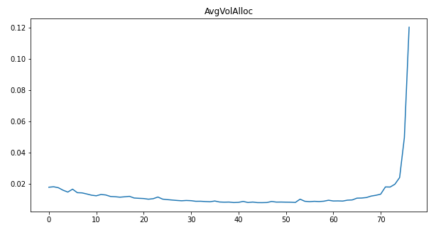
This is almost identical to the paper’s empirical result. We see that the trade volume grows exponentially as we near the end of the regular trading hours.

Average Correlation

Correlation and average correlation are defined as: \(\begin{align*} &\text{Correl}_{ijt} := { \sum_{d=1}^D (\text{DVol}_{idt} - \overline{\text{DVol}}_{it}(\text{DVol}_{jdt} - \overline{\text{DVol}}_{jt}) \over \sqrt{ \sum_{d=1}^D (\text{DVol}_{idt} - \overline{\text{DVol}}_{it})^2 - \cdot \sum_{d=1}^D (\text{DVol}_{jdt} - \overline{\text{DVol}}_{jt})^2}} \\ & \text{AvgCorrel}_t := {1 \over N(N-1)} \sum_{i \neq j} \text{Correl}_{ijt} \end{align*}\)

Again, this is pretty simple to compute in python as shown below:

correl = np.zeros((T, N, N))
for t in range(T):
    correl_num_t = np.array([(dvols[d, :, t] - bar_dvol[:, t]).reshape(-1, 1) 
                             @
                             (dvols[d, :, t] - bar_dvol[:, t]).reshape(-1, 1).T
                            for d in range(D)])
    correl_num_t = np.sum(correl_num_t, axis=0)
    
    var = np.array([np.square(((dvols[d, :, t]+1e-15)-bar_dvol[:, t]).reshape(-1, 1)) 
                           for d in range(D)])
    
    var = np.sum(var, axis=0)
    correl_denom_t = np.sqrt(var @ var.T)
    correl_t = correl_num_t / (correl_denom_t)
    correl[t, :, :] = correl_t
    
avg_correl = (1 / (N * (N-1))) * np.sum(correl, axis=(1, 2))

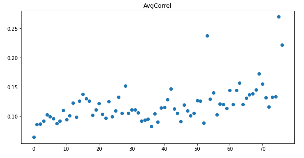
We see that the average correlation increases as we near 16:00. Note that our correalation values are much higher than those in the paper. This is mostly due to the fact that the paper used 459 S&P stocks (listed at both Nasdaq exchange and NYSE exchange) that contain many different market sectors such as technology, healthcare, energy, real estate, and so on. On the other hand, since we only used 147 stocks listed at the Nasdaq exchange and since most Nasdaq listed stocks are tech-related, they have higher correlation. We hypothesize the jump in correlation we see at interval near 55 is from FOMC/FED meeting, which happens near that time, but this needs some further research.

Decomposition of average volume allocation

Finally, we come to the main part of the paper. The paper assumes that there are two types of investors - single-stock and index-fund investors. Of course this is a huge generalization since there are other players in the market such as high frequency traders, liquidity providers, and so on. Such generalization was done to make analysis easier, and more importantly, it can serve as a baseline for a more complicated model.

Let \({\mathbf{\Psi}}_{id,t} :=\text{diag}(\psi_{id, 1t}, \psi_{id, 2t}, \cdots, \psi_{id, Nt})\) and \(\mathbf{\Psi}_{f,t} = \text{diag}(\psi_{f, 1t}, \psi_{f, 2t}, \cdots, \psi_{f, Nt})\) be single-stock and index-fund’s natural liquidity at interval $t$, and $\overline{\mathbf{\Psi}}_{id}$ and $\overline{\mathbf{\Psi}}_f$ be single-stock and index-fund’s total daily liquidty:

\[\overline{\mathbf{\Psi}}_{id} := \sum_{t=1}^T \mathbf{\Psi}_{id, t}, \quad \overline{\mathbf{\Psi}}_f := \sum_{t=1}^T \mathbf{\Psi}_{f,t}\]

In order to find the optimal policy, we want to model how the intensity of liquidity varies at each interval. Let single-stock investors’ liquidity $\psi_{id, it}$ vary over time $t=1, \dots, T$ according to profile $\alpha_t$, and index-fund investors’ liquidity $\psi_{f,kt}$ to vary according to another profile $\beta_t$:

\[\mathbf{\Psi}_{id, t} = \alpha_t \overline{\mathbf{\Psi}}_{id}, \quad \mathbf{\Psi}_{f,t} = \beta_t \cdot \overline{\mathbf{\Psi}}_f \quad \text{ for } t = 1, \dots, T\]

Since we do not know the total liquidity of single stock investor and index-fund investor, we need to make some assumptions to find them. The paper posits a simple generative model of single stock and portfolio order flow driven by two underlying Poisson processes. If $\theta_i$ denotes the fraction of the traded volume in a day for stock $i$ that is generated by order flow submitted by index fund investors:

\[\theta_i := {|\tilde{\omega}_{1,i} \cdot \bar{q}_f| \over \bar{q}_{id, i} + |\tilde{\omega}_{1i}| \cdot \bar{q}_f}\]

where \(\bar{q}_f\) is the notional traded by portfolio investors, \(\tilde{w}_{1i}\) is the weight of security $i$ in the index fund, \(\bar{q}_{id,i}\) is the notional traded by single stock investors in security $i$. For simplicty we assume that $\theta_1= \theta_2 = \cdots = \theta_N = \theta$.

Using the above model we get th efollowing intraday volume and pairwise correlation profiles:

\[\text{AvgVolAlloc}_t := {1 \over N} \sum_{i=1}^N {\mathbb{E}[\text{DVol}_{idt}] \over \sum_{s=1}^T \mathbb{E}[{\text{DVol}_{ids}}]} = \alpha_t \cdot (1-\theta) + \beta_t \cdot \theta\] \[\text{AvgCorrel}_t := {1 \over N(N-1)} \sum_{i\neq j} \text{Correl}_{ijt} = {\beta_t \cdot \theta^2 \over \alpha_t \cdot (1- \theta)^2 + \beta_t \cdot \theta^2}\]

Deriving the above result requires some work; luckily, most proofs are provided in the appendix. I will try to cover some proofs in a different post. For now we will focus on computing them using our empirical data from Nasdaq totalviewitch. Since we have already computed the empirical average volume allocation and average correlation, we need to find $\alpha_t$ and $\beta_t$ for all $t \in T$ that fits our empirical results. We can do this by setting up the equations as

\[\alpha_t \cdot (1-\theta) + \beta_t \cdot \theta = c_t \quad t = 1, \dots T\] \[{\beta_t \cdot \theta^2 \over \alpha_t \cdot (1- \theta)^2 + \beta_t \cdot \theta^2} = k_t \quad t = 1, \dots, T\] \[\sum_{t}^T \alpha_t = \sum_{t}^T \beta_t = \sum_{t}^T c_t = 1\] \[0 < \theta < 1\]

where $c_t$ and $k_t$ are the empirical results and we want to solve it for $\alpha_1, \dots, \alpha_T$, $\beta_1, \dots, \beta_T$. Initially, I tried tackling this problem using convex optimization approach until I found out that we can reduct this to a single univariate rational equation (mathematics stackexchange post).

To reduce it into a form we can plug into our solver, first let $\alpha_t = (1-\theta)\alpha_t$ and $b_t = \theta \beta_t$, then each pair of equations can be formed into a linear system of $a_t$ and $b_t$:

\[\begin{cases} a_t + b_t = c_t \\\theta b_t = k_t ((1- \theta)a_t + \theta b_t) \end{cases} \Leftrightarrow \begin{cases} a_t + b_t = c_t \\ (1-k_t)\theta b_t = k_t(1-\theta) a_t \end{cases}\]

Eliminating $b_t$ between equations:

\[(1-k_t) \theta (c_t - a_t) = k_t(1-\theta) a_t \Leftrightarrow a_t = {(1-k_t)c_t \theta \over (1-2k_t)\theta + k_t}\]

Substituting the above in $\sum_{t} \alpha_t = 1$ gives the eqaution in $\theta$:

\[\begin{align*} 1 = \sum_{t=1}^T \alpha_t &= \sum_{t=1}^T {a_t \over 1-\theta} \\ &= \sum_{t=1}^T {(1-k_t)c_t \theta \over (1-\theta)((1-2k_t)\theta + k_t)} \\ &= {\theta \over 1-\theta} \sum_{t=1}^T { (1-k_t)c_t \over (1-2k_t)\theta + k_t} \quad \cdots (*) \end{align*}\]

So we want to solve the equation $(*)-1 = 0$ which has a root $\theta \in (0, 1)$. Using scipy’s solver tools, we can plug in the above equation and get the result:

from scipy.optimize import root, least_squares 
import functools
def func(p):
    theta = p[0]
    # all RHS have to be 0
    e = [(1-avg_correl[i]) * avg_vol_alloc[i] / ((1-2*avg_correl[i])*theta + avg_correl[i])\
        for i in range(T)]
    s = functools.reduce(lambda a, b: a + b, e)
    f = theta / (1 - theta) * s - 1
    return f

params = [0.25] # theta starting point
sol = root(func, params)
theta = sol.x
alpha = (1/(1-theta))* (1-avg_correl) * avg_vol_alloc * theta /\
            ((1-2*avg_correl)*theta + avg_correl)
beta = (avg_vol_alloc - (1-theta) * alpha) / theta

Running this we get $\theta \approx 0.28184121$ which implies that about $28\%$ fo total traded volume orginate from the index fund. Let’s see what the plot looks like:

Intraday Trading Activity Profile

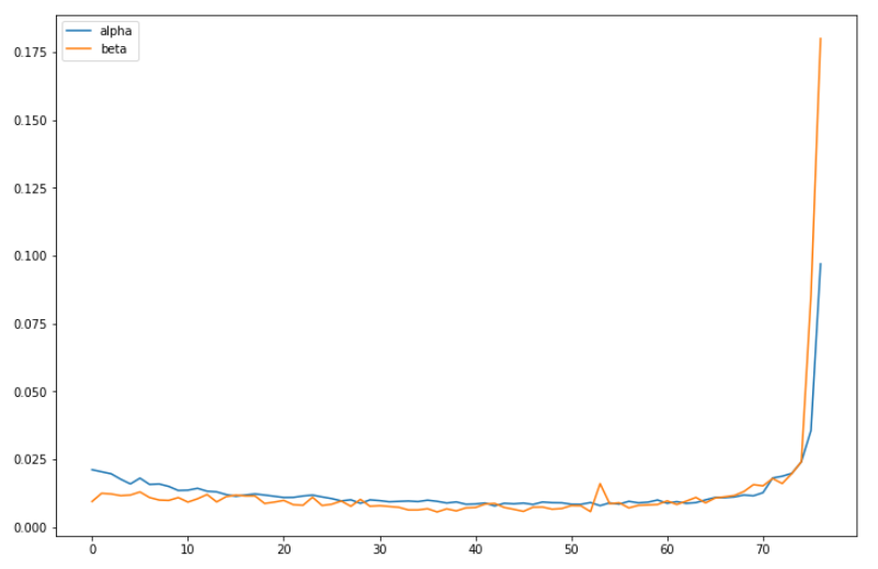
The above chart shows the intensity of trading volume between We see that the beginning of the trading day, the trading activity of index-fund investors $\beta_t$ is smaller than that of single-stock investor $\alpha_t$. But as we near the closing hours, $\beta_t$ completely dominates $\alpha_t$. This makes sense as we have empirically shown that pairwise correlation increased toward the end of the trading day, which is often the result of index-fund investors trading a basket of stocks.

Intraday Trading Activity Profile

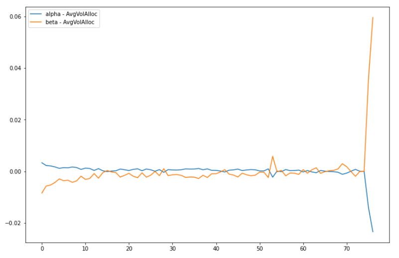
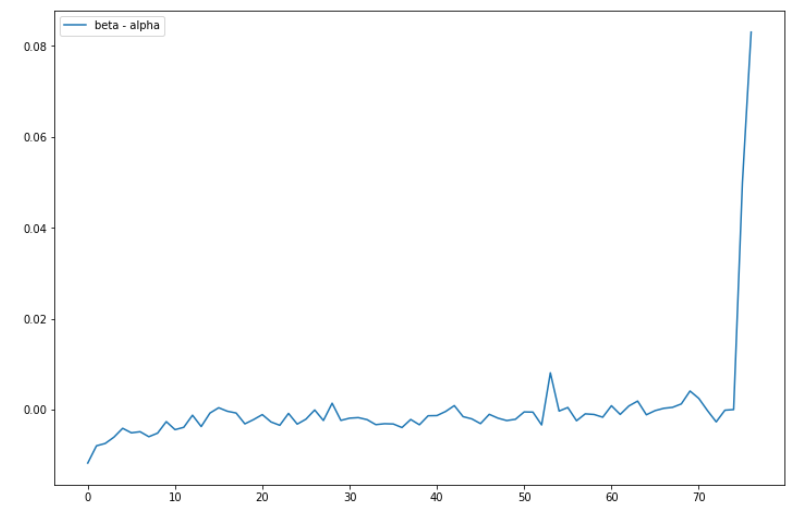
The above figure shows the deviation of $\alpha_t$ and $\beta_t$ from the market profile average volume allocation at $t$. Again, these values are slightly larger than the ones shown in the paper because of small sample size and lack of diversity.

Intraday Trading Volume

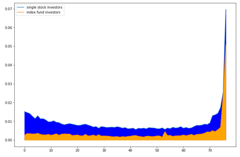
The above figure shows the intraday trading profiles $\alpha_t \cdot (1-\theta)$ and $\beta_t \cdot \theta$.

Proportion of Trading Volume

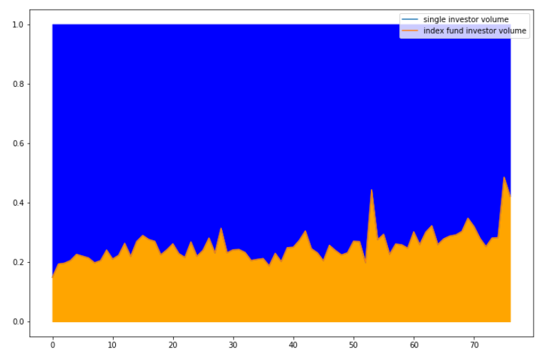
The above figure shows the proportion of index-fund order flows ${\beta_t \cdot \theta \over \alpha_t \cdot (1-\theta) + \beta_t \cdot \theta}$.

Difference in intraday Trading Activity Profiles

Lastly, the above fiture shows the effect of using optimal execution schedule. Since $\alpha_t > \beta_t$ in the morning, we want to execute in a separable VWAP-like execution. On the other hand, to exploit the increased end of the day liquidity and pairwise correlation of stocks, we want to avoid separable execution schedules and instead trade multiple stocks that align with index portfolios.

Final Remark

While I covered the nuts and bolts of the paper and shared my implementation, there is still a lot of details I have omitted. The paper is almost 40 pages including the appendix and contains lots of proofs (mostly linear algebra). I found most proofs to be strightforward but there are a couple of proofs that was not trivial. Overall, I found the paper to be very interesting. In future posts, I will try to go over some of them.